Author Archives: Gordon Rogers

Improved cool room design and maintenance

There are a number of ways of reducing energy requirements of cool stores.  Perhaps the most important is regularly checking the operating temperature of the room and considering whether this is the most cost-effective temperature for storage. For example, although the optimum storage temperature for many (non-chilling sensitive) products is close to zero, if they are only being stored for a short time then higher temperatures may be just as good. Monitoring the temperature will also indicate how often the system is defrosting and whether the cooling system is working effectively given external and internal heat sources.

Other possibilities include;

  • Pre-cooling product before it is placed in storage reduces heat load on the equipment and permits use of a smaller refrigeration plant. It can be more energy efficient to pre-cool with forced air in one room, then transfer product to a less regularly accessed second cool room for longer term storage.
  • Defrost the system regularly – ice build up on the evaporator greatly reduces efficiency. However, defrost cycles which overheat the air inside the cool store are also not desirable.
  • In some areas it may be possible to focus on cooling well insulated, fully packed stores at night using off-peak power. During the day they can be fully sealed.
  • Reduce fresh air exchange as much as possible – keep the door shut as much as possible, ensure door seals work well and check how air circulates through the cooling system
  • Use LEDs for lighting and turn lights off when not in use
  • Reflective paints applied to the outside of cool stores can reduce external heat load
  • Ensure cool room insulation is intact – damp insulation is no longer insulating


CO2 as a refrigerant gas

Using CO2 as a refrigerant gas can reduce energy consumption and increase cool room efficiency.

Refrigeration plant is generally a mature technology. Several refrigerants are in common use including R22 (being phased out due to its ozone depleting potential), R134a and R404a.

Although the refrigerants R134a and R404a do not significantly affect ozone depletion they have high global warming potentials (GWPs) of 1,300 and 3,260 CO2-e respectively. From 1st July 2012 synthetic refrigerant are taxed using the current carbon price and the above GWPs.

Perhaps surprisingly, CO2 itself has negligible greenhouse gas impact compared to synthetic refrigerants. As it has excellent heat transfer properties, smaller evaporator and condenser systems can be used to provide similar cooling to synthetic refrigerants. The drawbacks are a currently lower coefficient of performance (COP), mainly due to the less developed compressor technology, as well as its higher pressures needed which increase system cost.

CO2 has been used as a refrigerant for decades, but demand has only recently increased due to issues with synthetic refrigerants. It is increasingly used in Europe and there are some limited examples of its use in Australia, but apparently none in the vegetable industry.

Note that the CO2 system does not release CO2 into the cool room, it is contained within the sealed refrigeration system.

Comparison of refrigeration costs

Growers thinking of investing in new refrigeration plant will most likely compare the cost of continuing with their current system compared to the total cost of new equipment. The example shown below compares the net present value of three refrigeration plants; a paid off plant running on R134a, a new plant running on R134a and a new plant running on CO2.

R134a
new plant
R134a
paid off
CO2
new plant
min max min max min max
Total plant cost ($/kW_e) 500 1,000 550 1,250
Coefficient of performance (refrigerating power per unit of electrical energy) 3.0 2.5 2.5 2.0 2.5 2.0
Refrigerant price ($/kg) 50 100 50 100 10 50
Refrigerant price with carbon tax ($/kg)
NB Although price rises have been blamed on the carbon tax, this is a contentious issue with some refrigerant suppliers accused of price gouging)
80 130 80 130 10 50
Total plant cost including refrigerant ($/kW_e) 580 1,108 67 87 558 1,283
Electricity price ($/MWh) 200 300 200 300 200 300
Capacity factor (power consumed by the plant compared to its rated maximum capacity) 20% 25% 20% 25% 20% 25%
Annual electricity costs ($ per kW_e/year) 438 657 438 657 350 657
Leakage rate (%/year)
NB. Leakage of 10-15% is common, but a well maintained plant should leak less than this.
0 30 0 30 0 30
Leakage costs ($ per kW_e/year) 0 32 0 26 0 10
FOM 25 25 25 25 25 25
Total annual running cost ($ per kW_e/year) 463 714 463 708 375 692
Discount rate 0.05 0.1 0.05 0.1 0.05 0.1
Total net present value ($ per kW_e) 5,306 6,434 4,806 5,385 4,447 6,517

This analysis shows that the paid-off R134a plant is likely to cost in the order of $5,096/kW_e compared to $5,870/kW_e for a new R134a plant or $5,482/kW_e for a new CO2 plant. However, if the CO2. plant is able to achieve a lower capacity factor due to its better heat transfer, it may already be the most cost effective option. Although a new CO2 plant is currently 10-25% more expensive than a new R134a plant, this difference is likely to disappear within the next 15 years.

Importantly, refrigerant replacement represents a small component of total cost in all cases, even if R404a (with its higher global warming potential) is used and leakage rates were up to 30%. Electricity accounts for more than 80% of operating costs. Plant costs are secondary, with refrigerant replacement, operating and maintenance together accounting for roughly 10% of net present value.

A lesser known feature of CObased refrigeration is that it has a high temperature of heat rejection – roughly 120ºC. Recovering this waste heat may be useful, especially if large quantities of hot water are required to, for example, heat a greenhouse or manufacture a processed product. The financial viability of a CO2 based refrigeration plant is significantly improved if such waste heat can be used on-site.

As COplant improves it will become a better option.  Modelling for 2030 indicates that by then this technology will outperform synthetic refrigerants. Again, this is not because of the carbon price, but rather because of savings in electricity costs.


Efficient irrigation pumps

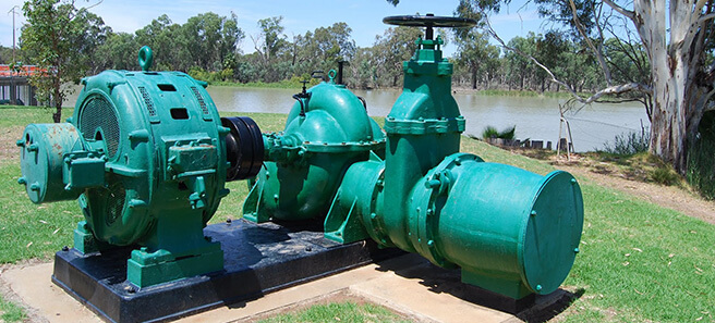
The pump is the heart of the irrigation system. Making sure it is the right pump for the job and that it is working properly can save energy costs.  But across the irrigation industry typically half of all pumps are found to be not operating efficiently. As a result energy costs are higher than they need to be.

The pump performance is determined by both the pump and motor performance. As shown below, pump performance is more important than the motor in determining net efficiency .  Typical improvements in the efficiency of the pump reduce the daily energy use by 19% and cost by $7.91/ML; typical improvements in the efficiency of the motor reduce the daily energy use by 3% and costs by only $0.80/ML.

Improving only pump efficiency Improving only motor efficiency
Pump 1 Pump 2 Pump 3 Pump 4
Pump efficiency 65% 80% 80% 80%
Motor efficiency 91% 91% 90% 93%
KW at pump 36.2 29.4 29.4 29.4
KW at meter 39.8 32.3 32.7 31.7
KW/h 39.8 32.4 32.7 31.6
Runtime (h/day) 16 16 16 16
Total KWh/day 637 518 523 506
Cost per day $97.20 $78.98 $79.85 $77.28
Cost per ML $42.19 $34.28 $34.66 $33.54

Working out the operating cost and efficiency of existing pumps is reasonably straightforward – See “How efficient is your pump” (NSW DPI), “Selecting the right pump for an irrigation system” (Ag WA) or “Pumping efficiency” (Growcom) for more information.

The pump

Pump efficiency will be determined by how well the pump duty (flow rate and operating pressure) is matched to the requirements of the irrigation system. If this is wrong then costs will mount quickly.

The original design should include information on the system flow-rate and pressure and how efficiently the pump operates under these conditions, as indicated by the pump curve. Once a pump is installed the operating conditions can be measured.

It is good practice to measure pump efficiency in the commissioning phase of new systems to ensure the system, including the pump, is working as specified. This can pick up any problems and ensure energy use and running costs are minimised.  Problems can include suction pipe diameter too small, lift too great and air entering the system (cavitation). These problems can drastically impact on a pump’s performance.

Over time a pump’s efficiency will decrease. By periodically measuring the pump’s efficiency and comparing this to the manufacture’s pump curve, the grower can decide when repair or replacement is cost-effective. This decision will involve a trade-off between increased energy use, and hence running costs, and the capital cost of the repair or replacement.

Appropriate maintenance is also required to maintain the efficiency of the pump. Problems with pumps can occur in the suction line, such as a blocked inlet, or a pipe damaged or crushed, or a build-up of deposits. On the pump, worn impellers and bearings, and seal and gland losses can all reduce the pump’s efficiency. Having a maintenance schedule and monitoring the performance of the pump will ensure these losses in performance remain at a tolerable level.

In summary, pump efficiency can be maximised by matching the pump to the irrigation system, good design of the pump station and regular maintenance. As a general rule, pump efficiency should be greater than 70% at duty; below this is poor. If you can get better than 80% this is excellent, with a maximum of 88% achievable in the field for an end-suction pump.

irrigation pump 1923

The pump motor

Electric motors increase in efficiency as they near full load. An electric motor operating at only 50% of full load will not be as efficient as one operating at close to 100% of full load. Aiming to have a motor that runs as close as practicable to full load can increase motor efficiencies by 2 to 5%.

As of Oct 2001 all three-phase electric motors from 0.73 to 185 kW, either manufactured or imported into Australia, must comply with minimum energy performance requirements as set out in AS/NZS 1359.5‐2000. This regulation was made even more stringent in April 2006, when the previous high-efficiency level became the new minimum standard. As a result all post-2006 three-phase electric motors are typically 2 – 3% more efficient than those manufactured before 2001.

Most irrigation pumps run at full speed no matter the load on the system. This can be very inefficient, particularly when a wide range of flow rates and pressures are needed, e.g. where flow rate varies due to different irrigation types or varying block size, or pressure varies considerably. A more energy-efficient system uses a variable speed drive to slow the motor speed to match the varying end-use requirements. If the irrigation-system flow rate or pressure does vary then variable speed drivers can reduce energy use.